Methodology Overview#
This package implements Echo State Networks (ESNs), which were introduced by Jaeger [2001]. ESNs are a Recurrent Neural Network architecture that are in a class of techniques referred to as Reservoir Computing. One defining characteristic of these techniques is that all internal weights are determined by a handful of global or “macro-scale” scalar parameters, thereby avoiding problems during backpropagation and reducing training time dramatically.
This page describes our two ESN implementations. First is a “standard” ESN architecture that is useful for small systems that can easily fit into memory on a computer. Second is a distributed ESN architecture that can be used for larger scale systems.
Standard ESN Architecture#
The basic ESN architecture that is implemented by the xesn.ESN class
is defined by the following discrete timestepping equations:
Here \(\mathbf{r}(n)\in\mathbb{R}^{N_r}\) is the hidden, or reservoir, state,
\(u(n)\in\mathbb{R}^{N_\text{in}}\) is the input system state, and
\(\hat{\mathbf{v}}(n)\in\mathbb{R}^{N_\text{out}}\) is the estimated target or output system state, all at
timestep \(n\).
The sizes of each of these vectors is specified to xesn.ESN via the
n_reservoir, n_input, and n_output parameters, respectively.
This form of the ESN has a “leaky” reservoir,
where the leak_rate parameter \(\alpha\)
determines how much of the previous hidden state to propagate forward in time.
This ESN implementation is eager, in the sense that all of the inputs, network
parameters, targets (during training), and predictions are held in memory.
Also, this form of the ESN assumes a linear readout, i.e., we do not transform the hidden state nonlinearly or augment it with the input or output state before passing it to the readout matrix. This choice is made based on testing by Platt et al. [2022], who showed that doing either of these two operations provided no additional prediction skill over a simple linear readout.
Internal Weights#
The adjacency matrix \(\mathbf{W}\in\mathbb{R}^{N_r \times N_r}\), the input matrix \(\mathbf{W}_\text{in}\in\mathbb{R}^{N_r \times N_u}\), and the bias vector \(\mathbf{b}\in\mathbb{R}^{N_r}\) are initialized with random elements, and usually re-scaled. These three matrices are generated as follows:
where \(\rho\), \(\sigma\), and \(\sigma_b\) are scaling factors,
\(f(\cdot)\) and \(g(\cdot)\) are normalization factors,
\(\hat{\mathbf{W}}\) and \(\hat{\mathbf{W}}_\text{in}\) are randomly generated matrices,
and
\(\hat{\mathbf{b}}\) is a randomly generated vector.
Each of these components can be specified by the user via the
adjacency_kwargs,
input_kwargs, and
bias_kwargs
options passed to xesn.ESN.
As an example, it is common to use a very sparse adjacency matrix, \(\hat{\mathbf{W}}\), with nonzero elements chosen from a uniform distribution ranging from -1 to 1, and to normalize the matrix by its spectral radius. In many cases, the scaling factor is chosen to be close to 1. These options could be selected by choosing:
adjacency_kwargs={
    "factor": 0.99,
    "distribution": "uniform",
    "normalization": "eig",
    "is_sparse": True,
    "connectedness": 10,
}
As another example, in Smith et al. [2023] the authors used a dense input matrix with elements randomly chosen from a uniform distribution from -1 to 1, and normalized the matrix by its largest singular value. This could be achieved as follows:
input_kwargs={
    "factor": 0.5,
    "distribution": "uniform",
    "normalization": "svd",
}
with the factor=0.5 just for the sake of an example, and note that
is_sparse=False is the default if the option is not provided.
The options to the bias vector are even more simple, as there is no option for sparsity and there are no normalization options.
Note
Internally, all of the options shown above are passed to the
xesn.RandomMatrix and xesn.SparseRandomMatrix classes,
where the is_sparse option selects between the two.
Please see these two class descriptions for all available options, and
numerous examples for creating different matrices.
Also note that the number of rows and columns for each matrix and the length
of the bias vector are automatically chosen based on the sizes set within
the ESN.
Training#
The weights in the readout matrix \(\mathbf{W}_\text{out}\) are learned
during training, xesn.ESN.train(),
which aims to minimize the following loss function
Here \(\mathbf{v}(n)\) is the training data at timestep \(n\),
\(||\mathbf{A}||_F = \sqrt{Tr(\mathbf{A}\mathbf{A}^T)}\) is the Frobenius
norm, \(N_{\text{train}}\) is the number of timesteps used for training,
and \(\beta\) is a Tikhonov regularization parameter chosen to improve
numerical stability and prevent overfitting, specified via the
tikhonov_parameter option to xesn.ESN.
Due to the fact that the weights in the adjacency matrix, input matrix, and bias vector are fixed, the readout matrix weights can be compactly written as the solution to the linear ridge regression problem
where we obtain the solution from scipy.linalg.solve on CPUs or cupy.linalg.solve on GPUs. Here \(\mathbf{I}\) is the identity matrix and the hidden and target states are expressed in matrix form by concatenating each time step “column-wise”: \(\mathbf{R} = (\mathbf{r}(1) \, \mathbf{r}(2) \, \cdots \, \mathbf{r}(N_{\text{train}}))\) and similarly \(\mathbf{V} = (\mathbf{v}(1) \, \mathbf{v}(2) \, \cdots \, \mathbf{v}(N_{\text{train}}))\).
Distributed ESN Architecture#
It is common to use hidden states that are \(\mathcal{O}(10)\) to \(\mathcal{O}(100)\)
times larger than the target system dimension.
In applications that have high dimensional system states, it becomes
necessary to employ a parallelization strategy to distribute the target and
hidden states across many semi-independent networks.
xesn.LazyESN accomplishes this with a generalization of the algorithm introduced by
Pathak et al. [2018], where we use
dask to parallelize the
computations.
The xesn.LazyESN architecture inherits most of its functionality from
xesn.ESN.
The key difference between the two is how they interact with the underlying data
they’re working with.
While the standard ESN had a single network that is eagerly operated on in
memory, xesn.LazyESN distributes
multiple networks to different subdomains of a single dataset and invokes lazy
operations via the dask.Array API.
This process is described with an example below.
Example: SQG Turbulence Dataset#
We describe the parallelization strategy based on the dataset used by Smith et al. [2023], which was generated by this model, written by Jeff Whitaker, following [Blumen, 1978, Held et al., 1995] for Surface Quasi-Geostrophic turbulence. For the purposes of this discussion, all that matters is the size of the dataset, which is illustrated below, and more details can be found in Section 2 of Smith et al. [2023].
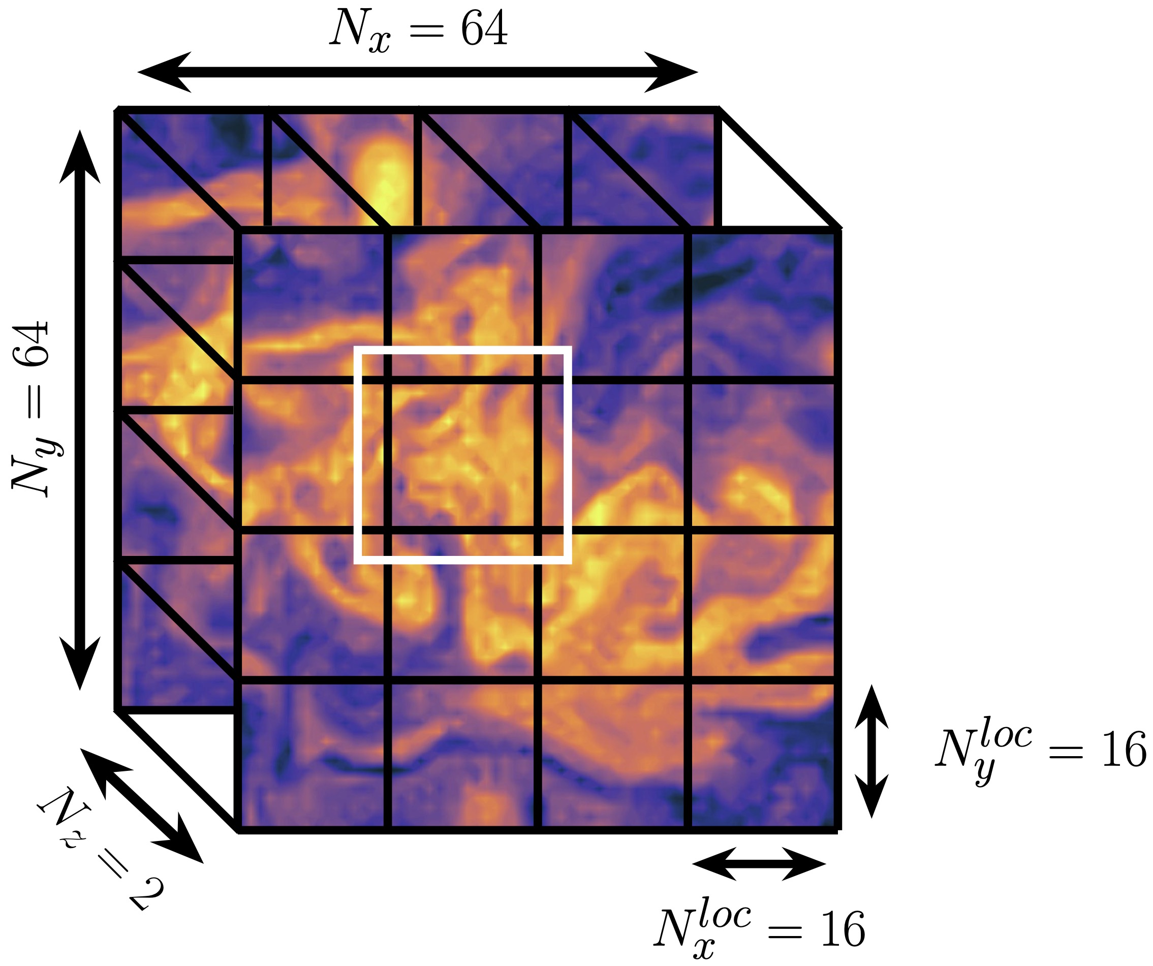
The dataset has 3 spatial dimensions \((x, y, z)\), and evolves in time, so
that the shape is \((N_x = 64, N_y = 64, N_z = 2, N_{time})\).
Parallelization is achieved in this case by subdividing
the domain into smaller chunks along the \(x\) and \(y\)
dimensions, akin to domain decomposition techniques in General Circulation
Models.
The subdivisions are defined by specifying a chunk size
to the model via esn_chunks.
In the case of our example, the chunk size is
esn_chunks={"x": 16, "y": 16, "z": 2}
and these chunks are denoted by the black lines across the domain in the figure
above.
Under the hood, xesn.LazyESN assigns a local network to each chunk,
where each chunk becomes a separate dask task.
Note that unlike xesn.ESN, xesn.LazyESN does not have
n_input and n_output parameters, but these are instead inferred from the
multi-dimensional chunksize, given by esn_chunks.
Communication between chunks is enabled by defining an overlap region, harnessing dask’s flexible overlap function (see this explanation in the dask documentation for additional description of this function). The overlap is defined by specifying the size of the overlap in each direction. For example
overlap={"x": 1, "y": 1, "z": 0}
defines a single grid cell overlap in \(x\) and \(y\), but no overlap in the vertical. Note that this argument is very similar to what can be provided to dask, except that the dimensions are labelled here, rather than numeral indices, due to our reliance on xarray. As an example, the overlap region is indicated by the white box in the figure above, where this overlap extends to both vertical levels for the chunk.
Note
Because of how xesn.LazyESN relies on dask chunks to define the
bounds of each distributed region, the time dimension is not allowed to be
chunked, nor can it have an overlap. That is, the size passed to
esn_chunks must be the size of the time dimension, or {"time":-1}
(shorthand).
The only option allowed for overlap is {"time":0}.
These are the defaults if nothing is provided for time as they are the only
acceptable options.
We have to tell the xesn.LazyESN how to handle overlaps on the
boundaries.
See here for
available options, since this is passed directly to dask’s overlap function.
In the case above, the domain is periodic in \(x\) and \(y\), so we can
simply write
boundary="periodic"
# or equally
boundary={"x": "periodic", "y": "periodic"}
Note once again that if a dict is used like the second case, then as with
overlap, the difference between what is expected here and with dask is that
the dimensions should be labelled, rather than provided as numeral indices.
One final option to xesn.LazyESN is persist. When dask arrays are
told to .persist() it means that they are brought into memory, using the
memory of the resources available (this means all data are brought into memory
if on a local machine).
In xesn.LazyESN, the persist option is a boolean, where if
True, then .persist() is called in the following places:
in
xesn.LazyESN.trainandxesn.LazyESN.predicton the input data, after calling dask’s overlap functionin
xesn.LazyESN.trainon the resulting readout matrix,xesn.LazyESN.Wout, after all computationsin
xesn.LazyESN.predicton the resulting prediction, after all computations
See this StackOverflow post for some discussion about persisting data, and see this page in the dask documentation for more information.
More Generally#
Here we make some notes for extending the description beyond this example. The dimensions that are chosen to be chunked (here \(x\) and \(y\)) should be first in the dimension order, and time needs to be last. Additionally, the time dimension needs to be labelled “time”, whereas the names of all other dimensions do not matter. Finally, currently only two dimensions are regularly tested, but the capability to add more could be added in the future.
Mathematical Definition#
The parallelization is achieved by subdividing the domain into \(N_g\) chunks, and assigning individual ESNs to each chunk. That is, we generate the sets \(\{\mathbf{u}_k \subset \mathbf{u} | k = \{1, 2, ..., N_g\}\}\), and where each local input vector \(\mathbf{u}_k\) includes the overlap region discussed above. The distributed ESN equations are
Here \(\mathbf{r}_k, \, \mathbf{u}_k \, \mathbf{W}_\text{out}^k, \, \hat{\mathbf{v}}_k\) are the hidden state, input state, readout matrix, and estimated output state associated with the \(k^{th}\) data chunk. The local output state \(\hat{\mathbf{v}}_k\) does not include the overlap region. Note that the various macro-scale paramaters \(\{\alpha, \rho, \sigma, \sigma_b, \beta\}\) are fixed for all chunks. Therefore the only components that drive unique hidden states on each chunk are the different input states \(\mathbf{u}_k\) and the readout matrices \(\mathbf{W}_\text{out}^k\). Additionally, because the solution to the ridge regression problem is linear, the readout matrices are simply:
where each readout matrix can be computed independently of one another.
Macro-Scale Parameters#
From our experience, the most important macro-scale parameters that must be specified by the user are the
input matrix scaling, \(\sigma\),
input_kwargs["factor"]adjacency matrix scaling, \(\rho\),
adjacency_kwargs["factor"]bias vector scaling, \(\sigma_b\),
bias_kwargs["factor"]Tikhonov parameter, \(\beta\),
tikhonov_parameterleak rate, \(\alpha\),
leak_rate
See this example for a demonstration of using the surrogate modeling toolbox to perform Bayesian optimization and find well performing parameter values.